State Space Models and the Kalman Filter [/ˈsteɪt ˈspeɪs ˈmɑdəlz ənd ðə ˈkælmən ˈfɪltər/] n - A state-space model parts what you observe from what you believe drives the observations. The state equation tells how an unobserved state evolves; the observation equation binds that state to the data you actually see.

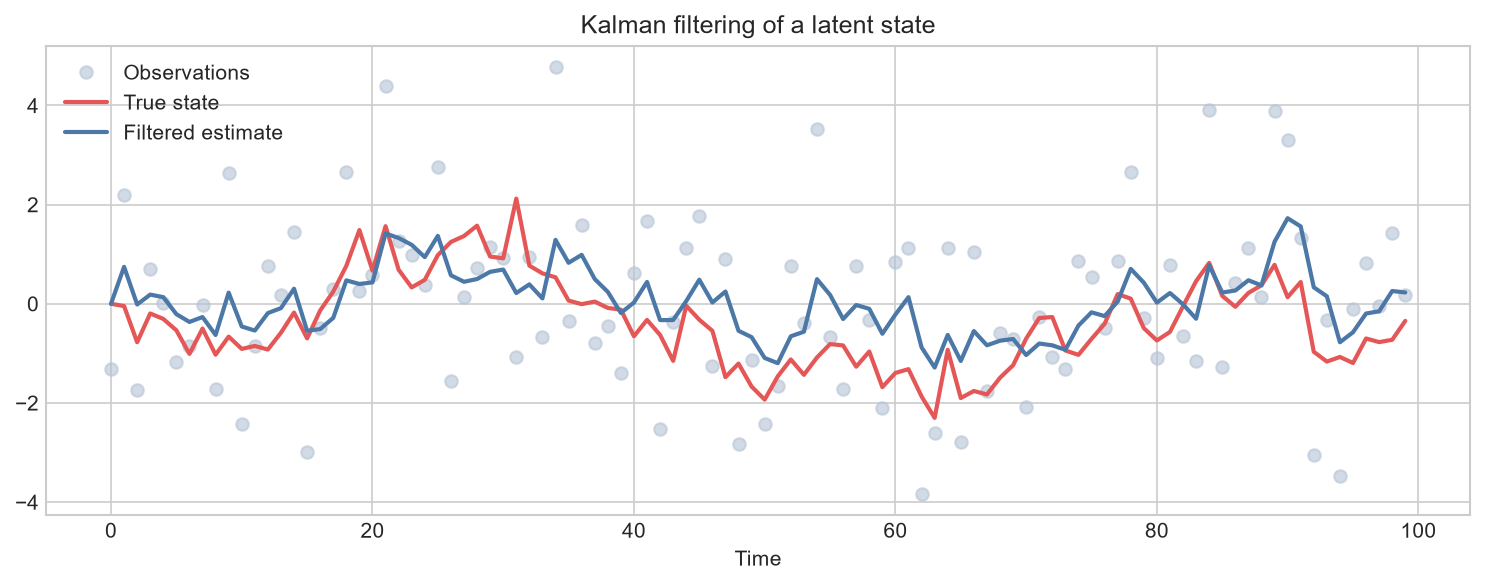Kalman filtering of a latent state

The linear Gaussian form is:

$$\begin{gathered} x_t=F{x}_{t-1}+w_t, \\ quad{w}_t \\ simN(0,Q) \end{gathered}$$ $$\begin{gathered} y_t=H{x}_t+v_t, \\ quad{v}_t \\ simN(0,R) \end{gathered}$$

$x_t$ is the latent state. $y_t$ is the observation. $F$ is the transition matrix, $H$ the observation matrix, and $Q$ and $R$ the process and measurement noise covariances.

The Kalman filter is a recursive contrivance that updates the state’s distribution as each new observation arrives, and it has two steps. In prediction, the state distribution is carried forward by the state equation; in update, the prediction is corrected by the new observation, according to the relative uncertainty of prediction against measurement.

The Kalman gain settles how much weight the new observation receives:

$$K_t=P_{t|t-1}{H}^T(H{P}_{t|t-1}{H}^T+R{)}^{-1}$$

When the measurement noise $R$ is small beside the prediction uncertainty, the gain runs high and the filter trusts the data. When $R$ is large, the filter trusts the model.

State-space models gather many seemingly distinct methods under one roof. ARIMA can be written in state-space form. Time-varying regression betas become a state-space model in which the coefficients are the latent state. Regime switching turns nonlinear once the state is discrete; see Regime Switching and Hidden Markov Models for that extension.

The practical difficulty is specification. Choose too little process noise and the filter ignores the data; choose too much and it overreacts. The noise covariances are usually estimated by maximum likelihood, which is to say they are estimated with error, like everything else.